Personal Project · Open Source

Gradient Optimizers
Built from Scratch

7 optimizers implemented in pure NumPy — from vanilla Gradient Descent to Adam — benchmarked on convex, ill-conditioned, and non-convex landscapes with full convergence analysis and a PyTorch DL benchmark.

7 Optimizers 4 Landscapes 3 LR Schedules NumPy from Scratch PyTorch Benchmark

GitHub Repo 📄 Full Report ← Portfolio

Results at a Glance

Key Numbers

Optimizers from scratch

5×

Speedup from Momentum on κ=100

98.5%

SGD+Nesterov test accuracy (make_moons)

O(1/k²)

Nesterov rate — confirmed empirically

Algorithms

Seven Optimizers

Gradient Descent

x = x − lr · ∇f(x). The baseline. Works well on easy problems, zigzags on ill-conditioned ones.

O(1/k)

SGD (mini-batch)

Noisy gradient from random mini-batch. Supports cosine, step decay, and warmup schedules.

Stochastic

Momentum

Accumulates velocity — dampens oscillations in ravines. ~5× faster than GD on κ=100.

β = 0.9

Nesterov AGD

Evaluates gradient at the look-ahead point. Provably optimal O(1/k²) rate — confirmed empirically.

O(1/k²) optimal

AdaGrad

Per-parameter adaptive lr using cumulative squared gradients. Stalls on dense gradient problems.

Adaptive

RMSProp

Fixes AdaGrad's vanishing lr via exponential moving average. Stays stable throughout training.

EMA · ρ = 0.9

Adam

Momentum + RMSProp + bias correction. Most robust across all landscapes — the safe default.

β₁=0.9 · β₂=0.999

Convergence Results

Experiment Outputs

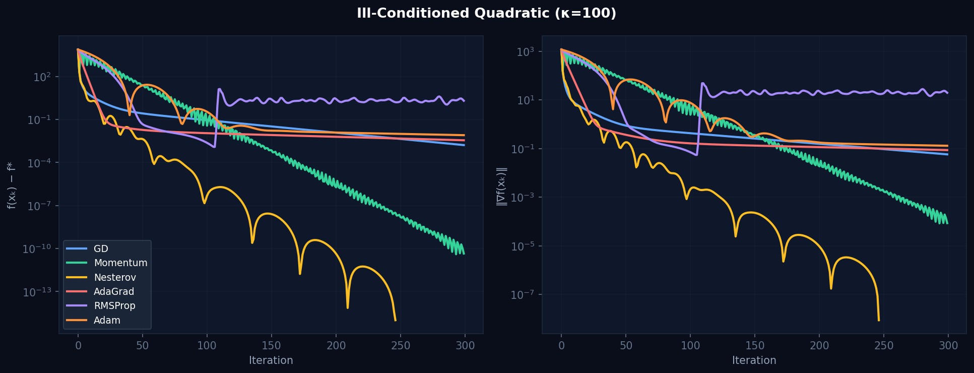
Figure 1. Ill-conditioned quadratic (κ=100) — suboptimality (left) and gradient norm (right). Adam and Nesterov converge in ~50–80 iterations; GD takes 300+ and still lags behind.

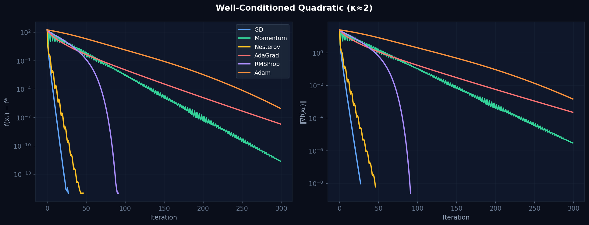
Figure 2. Well-conditioned quadratic (κ=2). All optimizers converge — differences are small. Nesterov and Adam reach machine precision earliest.

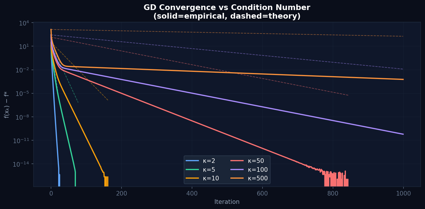
Figure 3. GD convergence vs condition number κ ∈ {2, 5, 10, 50, 100, 500}. Solid lines are empirical; dashed lines are the theoretical bound ((κ−1)/(κ+1))^k. κ=500 does not converge in 1000 iterations.

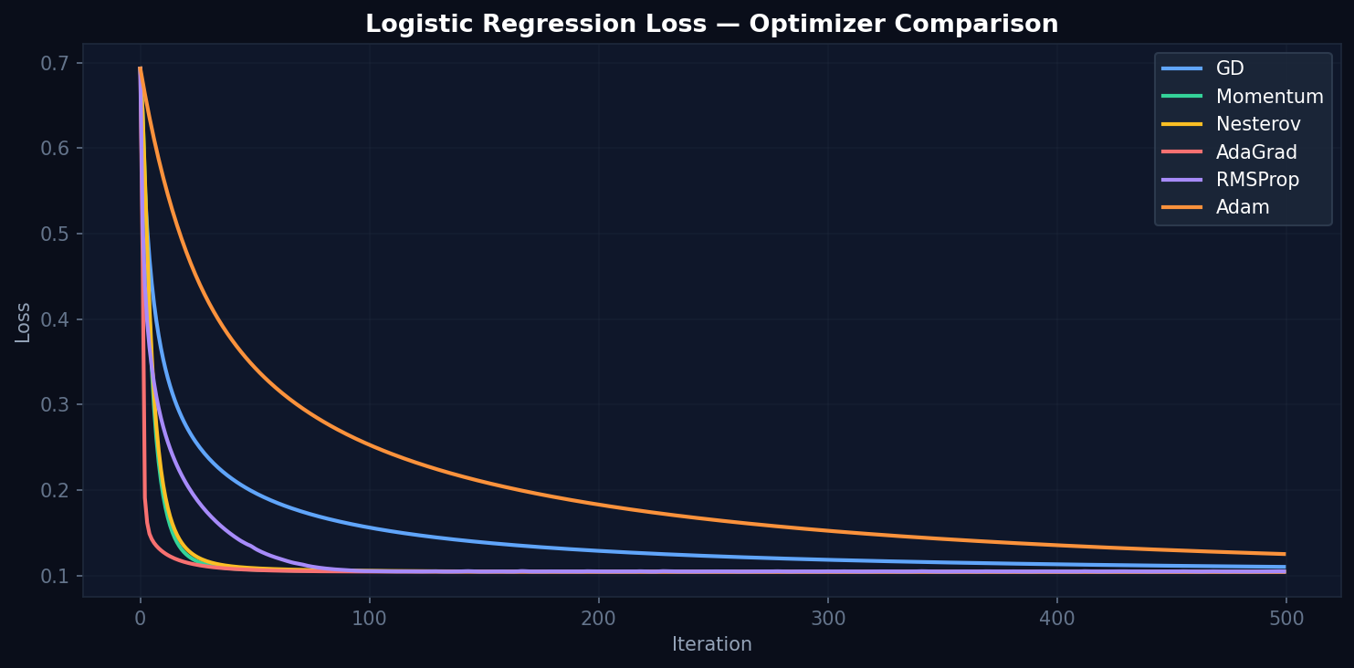
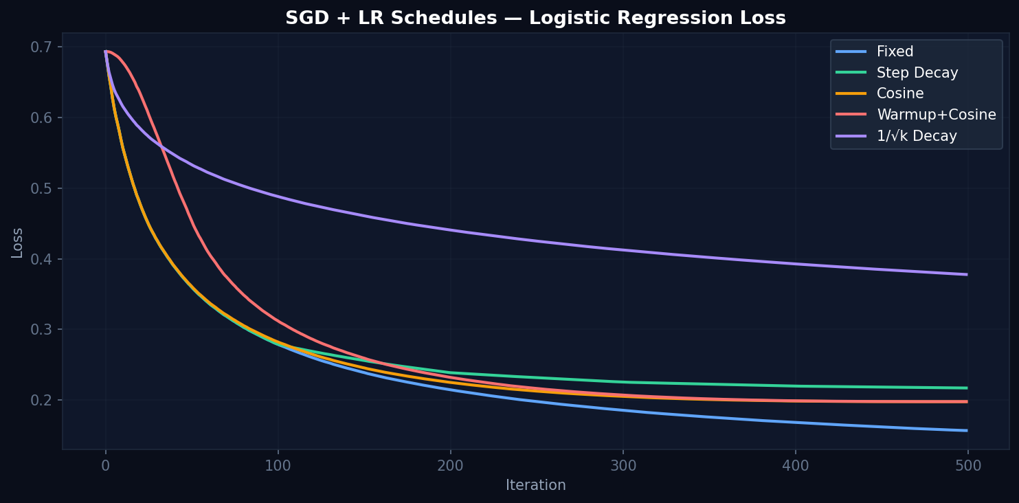
Figure 4. Logistic regression loss. Momentum, Nesterov, RMSProp reach ~0.10 within 100 iterations. Adam converges slowly here.

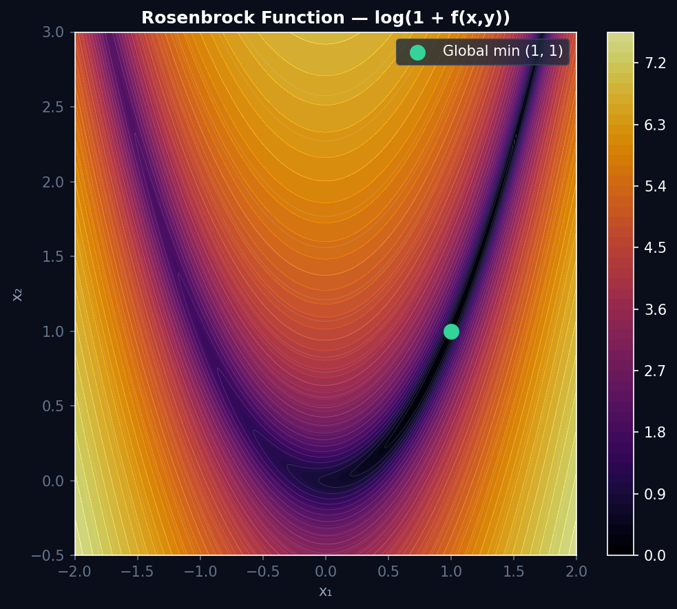
Figure 5. Rosenbrock landscape (log scale). The narrow banana-shaped valley curving toward the global min at (1, 1).

Learning Rate & Deep Learning

Schedule & Benchmark Results

Figure 6. SGD with 5 LR schedules on logistic regression. Fixed LR reaches lowest final loss (~0.155). Cosine and Warmup+Cosine reach ~0.20. The 1/√k schedule decays too fast and stalls at ~0.38.

Figure 7. MLP training and validation BCE loss on make_moons (200 epochs). Adaptive methods converge faster; SGD variants are smoother.

Figure 8. Test accuracy per optimizer. SGD, Momentum, Nesterov: 98.5%. Adam, RMSProp, AdaGrad: 97.5% — Adam's generalization gap on small datasets.

Takeaways

What the Experiments Showed

📐

Theory matches experiment exactly

GD empirical curves follow the bound ((κ−1)/(κ+1))^k precisely. At κ=500, GD cannot converge in 1000 iterations — theory predicts this.

🏎️

Momentum: 5× faster on κ=100

Adding β=0.9 momentum reduces iteration count from 300+ to ~60 on the ill-conditioned quadratic. One hyperparameter, massive practical effect.

🔭

Nesterov's look-ahead is real

The O(1/k²) optimal rate is confirmed empirically — Nesterov consistently outperforms plain momentum on every landscape tested.

⚠️

AdaGrad stalls on dense gradients

The cumulative squared gradient denominator grows forever, shrinking the effective lr to near zero within ~100 iterations on dense problems.

📅

Fixed LR beats cosine on logistic

Fixed LR reaches ~0.155 final loss vs ~0.20 for cosine annealing — the constant step size keeps descending while schedules slow down.

🎯

SGD beats Adam on accuracy

SGD+Momentum+Nesterov all hit 98.5% on make_moons. Adam/RMSProp/AdaGrad reach 97.5% — the Adam generalization gap is real even on small tasks.

Code

Quick Start

from src.landscapes import make_ill_conditioned_quadratic

from src.optimizers import run_all

import numpy as np, matplotlib.pyplot as plt

landscape = make_ill_conditioned_quadratic(n=10, kappa=100)

results = run_all(landscape, x0=np.zeros(10), n_iter=300)

for name, r in results.items():

    plt.semilogy(r.f_history, label=name)

plt.legend(); plt.xlabel("Iteration"); plt.show()

Python 3.10+ NumPy PyTorch Matplotlib Jupyter

Gradient Optimizers Built from Scratch